A Framework on Engineering Calculation With Units in Typst. Featured with unit and number formatting by zero package.
Installation
Import the package by
#import "@preview/pariman:0.2.2": *
Or install the package locally by cloning this package into your local package location.
Usage
For a comprehensive documentation, you can refer to the docs.
The quantity function
The package provides a dictonary-based element called quantity. This quantity can be used as a number to all of the calculation functions in Pariman’s framework. The quantity is declared by specify its value and unit.
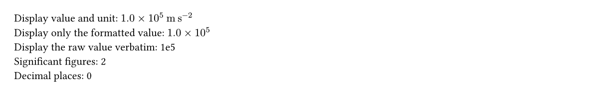
#let a = quantity("1.0e5", "m/s^2")
Display value and unit: #a.display \
Display only the formatted value: #a.show \
Display the raw value verbatim: #a.text \
Significant figures: #a.figures \
Decimal places: #a.places
Pariman’s quantity takes care of the significant figure calculations and unit formatting automatically. The unit formatting functionality is provided by the zero package. Therefore, the format options for the unit can be used.
#let b = quantity("1234.56", "kg m/s^2")
The formatted value and unit: #b.display  \
#zero.set-unit(fraction: "fraction")
After new fraction mode: #b.display

Pariman loads the zero package automatically, so the the unit formatting options can be modified by zero.set-xxx functions.
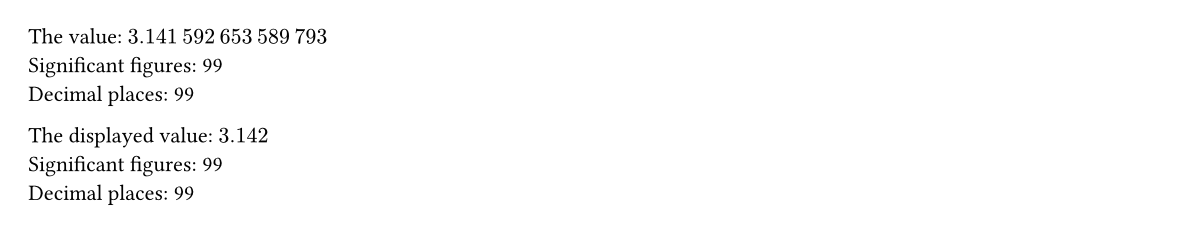
For exact values like integers, pi, or other constants, that should not be counted as significant figures, Pariman have the #exact function for exact number quantities. The #exact function does not accept unit and has 99 significant figures.
#let pi = exact(calc.pi)
The value: #pi.display \
Significant figures: #pi.figures \
Decimal places: #pi.places

// The shorter version
#let s-pi = exact(calc.pi, display-figures: 4)
The displayed value: #s-pi.display \
// does not effect the real significant figures
Significant figures: #s-pi.figures \
Decimal places: #s-pi.places
Note that the quantity function can accept only the value for the unitless quantoity.
The calculation module
The calculation module provides a framework for calculations involving units. Every function will modify the input quantitys into a new value with a new unit corresponding to the law of unit relationships.
#let s = quantity("1.0", "m")
#let t = quantity("5.0", "s")
#let v = calculation.div(s, t) // division
The velocity is given by #v.display. \
The unit is combined!

Moreover, each quantity also have a method property that can show its previous calculation.
#let V = quantity("2.0", "cm^3")
#let d = quantity("0.89", "g/cm^3")
#let m = calculation.mul(d, V)
From $V = #V.display$, and density $d = #d.display$, we have
$ m = d V = #m.method = #m.display. $
 The `method` property is recursive, meaning that it is accumulated if your calculation is complicated. Initially, `method` is set to `auto`.
#let A = quantity("1.50e4", "1/s")
#let Ea = quantity("50e3", "J/mol")
#let R = quantity("8.314", "J/mol K")
#let T = quantity("298", "K")
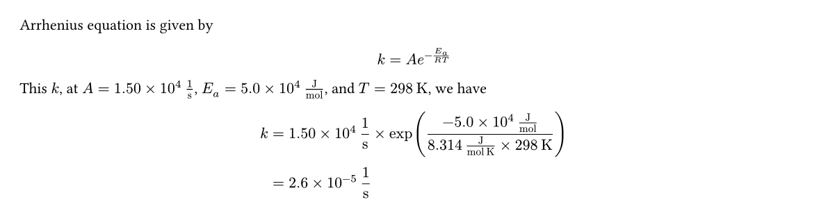
Arrhenius equation is given by
$ k = A e^(-E_a/(R T)) $
This $k$, at $A = #A.display$, $E_a = #Ea.display$, and $T = #T.display$, we have
#let k = {
import calculation: *
mul(A, exp(
div(
neg(Ea),
mul(R, T)
)
))
}
$
k &= #k.method \
&= #k.display
$
Sometimes, you may want to display your calculations with units omitted. The quantity function has a parameter explicit which is true by default. If this parameter is set to false, the unit of that quantity is ommitted for all of its calculation.
#let r = quantity("2.0e-5", "cm")
// hide the unit in `method`.
#let T = quantity(
"373", "K", explicit-method: false
)
#let M = quantity("28", "g/mol")
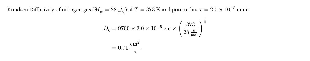
Knudsen Diffusivity of nitrogen gas ($M_w = #M.display$) at $T = #T.display$ and pore radius $r = #r.display$ is
#let D-K = {
import calculation: *
mul(
exact(9700), r, root(div(T, M), 2),
unit: "cm^2/s"
)
}
$ D_k &= #D-K.method \ &= #D-K.display $
set-quantity
If you want to manually set the formatting unit and numbers in the quantity, you can use the set-quantity function.
#let R = quantity("8.314", "J/mol K")
#let T = quantity("298.15", "K")

#calculation.mul(R, T).display
// 4 figures, follows R (the least).

// reset the significant figures
#let R = set-quantity(R, figures: 8)
#calculation.mul(R, T).display
// 5 figures, follows the T.

Moreover, if you want to reset the method property of a quantity, you can use set-quantity(q, method: auto) as
#let R = quantity("8.314", "J/mol K")
#let T = quantity("298.15", "K")
#let prod = calculation.mul(R, T)
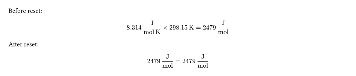
Before reset:
$ prod.method = prod.display $
// reset
#let prod = set-quantity(prod, method: auto)
After reset:
$ prod.method = prod.display $
Unit conversions
The new-factor function creates a new quantity that can be used as a conversion factor. This conversion factor have the following characteristics:
- It has, by default, 10 significant figures.
- It have a method called
invfor inverting the numerator and denominator units.
#let v0 = quantity("60.0", "km/hr")
#let km-m = new-factor(
quantity("1", "km"),
quantity("1000", "m")
) // km -> m
#let hr-s = new-factor(
quantity("1", "hr"),
quantity("3600", "s"),
) // s -> hr
#let v1 = calculation.mul(v0, km-m)
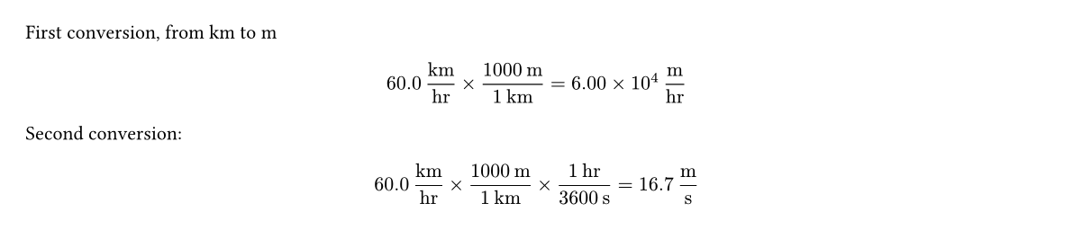
First conversion, from km to m
$ v1.method = v1.display $
// change from hr -> s, use `hr-s.inv` because hr is in the denominator
#let v2 = calculation.mul(v1, hr-s.inv)
Second conversion:
$ v2.method = v2.display $
In-Text Quantity Declaration (The qt Module)
This module provides a top-layer functions that makes declaration of the quantities can be done at the same time as showing the formatted quantities. Declaration can be done by qt.new() function, which receives the same argument set as the quantity constructor, but with an additional, positional argument: its key/name. This name is important because it will be used to retrieve the value declared for further calculations or updates.
// Syntax: #qt.new(name, value, ..units)
A chemist added #qt.new("mA", "1.050", "g")
of A into a beaker filled with
#qt.new("Vw", "100", "mL") of water.

Moreover, this #qt.new function also receives the following named options:
displayed(bool, default:true) Whether to display the declared quantity immediately.is-exact(bool, default:false) Whether to set the specified quantity as an exact value (like declaring byexactfunction). To manipulate the quantities declared, we can use#qt.update(key, function)to update the variable that has a namedkey(same as the name specified by#qt.new), or create a new quantity namedkeyby using a functionfunction. For example,
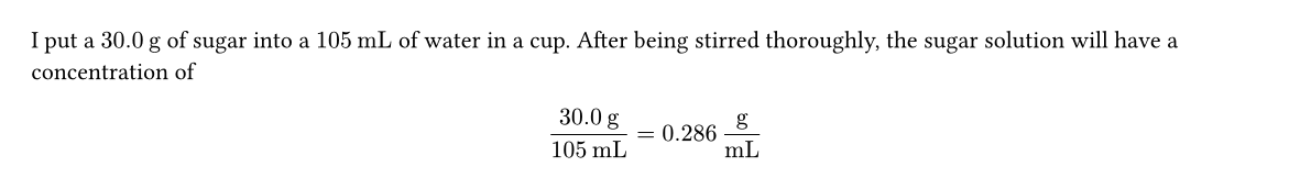
I put a #qt.new("ms", "30.0", "g") of sugar into a #qt.new("V", "105", "mL") of water in a cup. After being stirred thoroughly, the sugar solution will have a concentration of
// import the division function
#import calculation: div
// An update to calculate the concentration!
#qt.update("conc", q => div(q.ms, q.V))
// Show the result!
$ #qt.method("conc") = #qt.display("conc") $
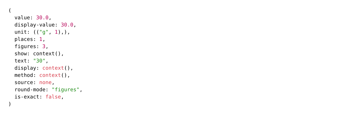
Note that #qt.display(key) and #qt.method(key) are used as shortcut for accessing the display and method properties of the quantity identified by the name key. For other properties, you can access by #qt.get(key: name) as the following. Highlight the context.
#context qt.get(key: "ms")
Lastly, you can set the property like set-quantity function by using the analogous #qt.set-property(key, ..properties), such as
What is the value of $pi$? \
// too long number!
It is #qt.new("pi", calc.pi, is-exact: true)  \
Oh, too long,  \
// set the displayed figure number
#qt.set-property("pi", display-figures: 4)
It is now only #qt.display("pi")
Available Calculation Methods
All functions in calculation module also accept the same format options in the quantity function for formatting the result quantity.
neg(a)negate a number, returns negative value ofa.add(..q)addition. Error if the unit of each added quantity has different units. Returns the sum of allq.sub(a, b)subtraction. Error if the unit of each quantity is not the same. Returns the quantity ofa - b.mul(..q)multiplication, returns the product of allq.div(a, b)division, returns the quantity ofa/b.inv(a)returns the reciprocal ofa.exp(a)exponentiation on based $e$. Error if the argumenrt of $e$ has any leftover unit. Returns a unitlessexp(a).pow(a, n)returns $a^n$. If $n$ is not an integer,amust be unitless.ln(a)returns the natural log ofa. The quantityamust be unitless.log(a, base: 10)returns the logarithm ofaon basebase. Error ifais not unitless.root(a, n)returns the $n$th root ofa. Ifnis not an integer, thenamust be unitless.solver(func, init: none)solves the function that is written in the formf(x) = 0. It returns another quantity that has the same dimension as theinitvalue.